The ATP Dataset and The Filthy Rich Tennis Players

After approximately an hour thinking about an interesting dataset to test what I’ve learned from my recent studies in Data Science and Machine Learning, all of a sudden, someone at home starts to watch the USOpen. Perfect, that’s exactly what I was looking for. But where can you find the data? Well, let’s go to the source: the ATP Singles Ranking website.

Unfortunately, that’s not enough to study a little bit more in-depth the patterns of the sport. We need a way of storing that data so we can manipulate it — although they do make some structured data available with some files, those are very superficial statistics —, we need web scraping. And that’s how we get to the outline of this article:

How to Get the Data
Analyzing the Data

I assume the first section is not for everybody, but, still, the second part has many interesting conclusions and you can just skip to it.

As is the norm, I’ve made all the source code for this article available in this ATP Github Repo and you can use it to get the stats for any given range of players and also from any date in time — comparing today’s statistics to the times of Sampras and Agassi should be interesting and probably a topic of a future article.

There are basically two ways of obtaining the necessary scraps from the .html files:

Parsehub
Python Web Scraping

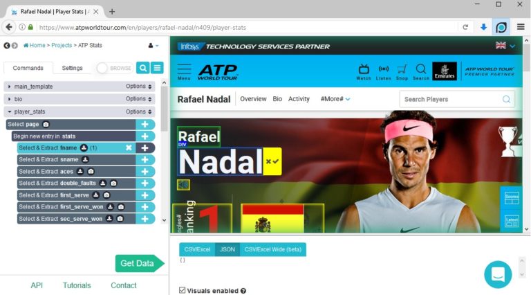
The first method is way more easy-going and friendlier, but also much more expensive and time consuming — in terms of downloading time. Parsehub is a paid software which will slow down the free version — and limit the amount of pages per run — on purpose just so you feel more inclined to pay for the complete package. The subscription ranges from US$150 for the standard version to US$500 for the professional — what pro would use that software when he can get much more data much faster via programming? — version, not at all cheap. Personally, I wouldn’t recommend it if you want to get a big dataset (more than 200 web pages), but if it’s a small amount of data, Parsehub will get you going very fast: they have good tutorials and a nice interface.

An example of project inside Parsehub. The selections are all through a graphical interface.

You could use basically any language you like for this, but I’ll use Python as it is very easy and has the very useful package BeautifulSoup, which will help us parse through the endless garbage the html files will throw at us. What I did to get the full data set is a bit too much for this article, but I’ll skim through some of the essential steps.

First, you will need to send a request for the singles ranking web page and then obtain all the links for each player’s web page, this way we will be able to loop around each player’s statistics. These steps would be condensed to:

          import requests
from bs4 import BeautifulSoup
N = 5
page_ranking = requests.get('https://www.atpworldtour.com/en/rankings/singles?rankDate=2018-08-27&rankRange=1-' \
+ str(N))
ranking = BeautifulSoup(page_ranking.content, 'html.parser')
ranking_list = list(ranking.findAll('td', {'class':'player-cell'}))
rank_url = []
for i in range(0, N):
  a = str(list(ranking_list[i])[1])
  b = 'https://www.atpworldtour.com' + \
        a[(a.find('href="')+6):(a.find('>')-1)].replace('overview','')
  rank_url.append([i+1,b])

As you can see from the for loop, web scraping does not yield the cleanest code in the universe, in fact, it looks very dirty, but you usually just can’t avoid it, you will have to find the html tag that contains the bit of text you need using the find() or findAll() methods and cut out the trash, which is inherently done case by case and mostly not pretty — a more experienced coder will certainly find better solutions than I do, but I doubt he will be able to always write clean code for this task. For example, next, we will need to parse the “overview” and “player-stats” web pages and, after using the list and str commands to make things easier to deal with — and to have normal Python objects instead of BeautifulSoup ones — we get the string: ' <tr>\n<td>\r\n\t\t\tBreak Points Converted\r\n\t\t</td>\n<td>\r\n\t\t\t41%\r\n\t\t</td>\n</tr>'. With that string, we can then select only the part we want, the percentage, with a slice like c = int(b[55:-16]). And that’s one of the easiest selections in this dataset.

          page_plrstats = requests.get(rank_url[1][1] + 'player-stats')
plrstats = BeautifulSoup(page_plrstats.content, 'html.parser')
a = plrstats.findAll('table', {'class':'mega-table'})
b = str(list(list(list(a)[1])[3])[7])
c = int(b[55:-16])

One last thing I would like to point out is that using the try and except Python blocks will make your life much easier. Sometimes the player will not have the data or might have an irregular formatting, so you don’t want to have errors popping out all the time. As an example, the basic cell in my code for this dataset is then:

          # Service Games Won
try:
  a = plrstats.find('table', {'class':'mega-table'})
  b = str(list(list(a)[3])[17])
  c = int(b[50:-16])
  player_dict['serve_won'] = c
except:
  print('serve won',i+1)

Both Parsehub and Python offer two very common file types for saving data: csv and json. You may choose the easiest for you, however, I highly recommend you use json, as it is way easier to organize the data and write better structures, sometimes csv’s can be marginally readable, csv is a bit too crude to my taste. After making a list of dictionaries, you have all the ingredients to save the data inside a json file, and this can be easily done with:

          import json
name = 'atp_python_1-' + str(N) + '.json'
with open(name, 'w') as f:
for dic in players:
json.dump(dic, f)
f.write('\n')

Later, opening the file is similarly easy:

          N = 1500
date = '2018-08-27'
name = 'atp_python_' + date + '_1-' + str(N) + '.json'
with open(name) as d:
players = [json.loads(line) for line in d]

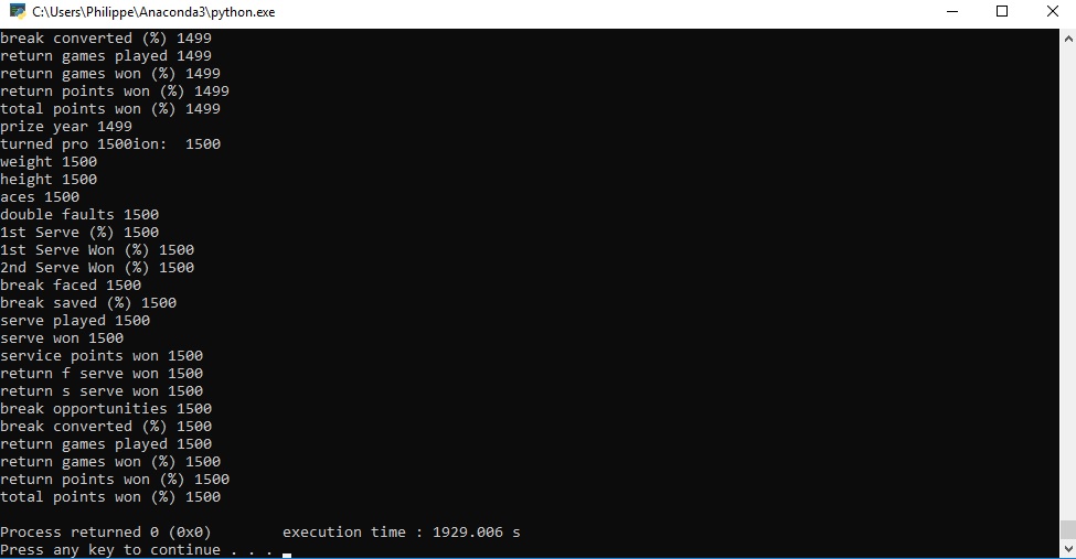
Extracting the whole dataset for the first 1,500 — I wouldn’t go much further than that, there is not a lot of data beyond rank 1,500 — players took me a bit more than half an hour, about 50 players per minute — don’t be afraid of the prints you get on the screen, they happen when the extractor couldn’t get that particular datum from the player, most likely because there wasn’t any.

This will only be a brief analysis, I’ll leave a more in-depth and complete one to other posts; nonetheless, the conclusions are still interesting. I believe that (my) the saying “sport is the epitome of society” will resonate very strongly with you after this brief discussion.

Let’s start with a graph of the prize in tournaments versus the rank of the player:

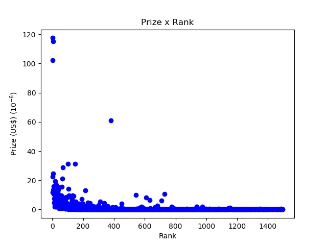
The top left dots are the filthy rich dominating players Rafael Nadal, Roger Federer and Novak Djokovic (and the dot around 60 million is Andy Murray). That graph shows us a huge disparity in the wealth distribution available to the players, much like society in general, where we have 1% (even less nowadays) of the people owning 99% of the wealth.

Let’s take out the four top grossing players to take a closer look at the bottom curve:

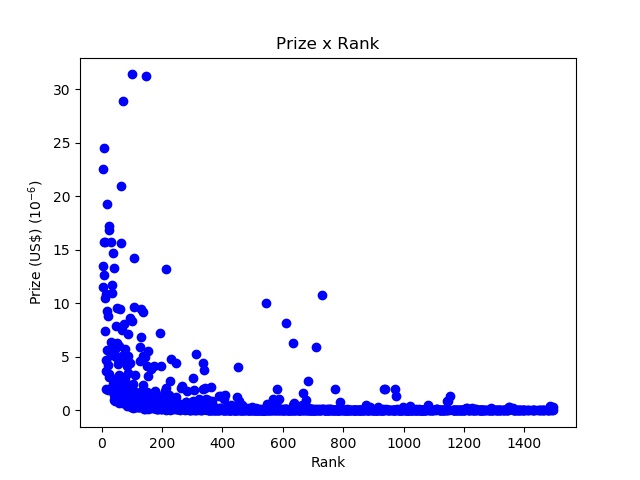
Prize (Millions of US$) x Rank (without Rafael Nadal, Roger Federer, Novak Djokovic and Andy Murray).

The shape is pretty close to an exponential curve with a very steep decay, again the heavy mark of inequality. I wouldn’t call the players from rank 400 and above poor, but the difference to the top is quite staggering.

Another useful graph to take into account is that of the sum of the prize money up to a certain rank:

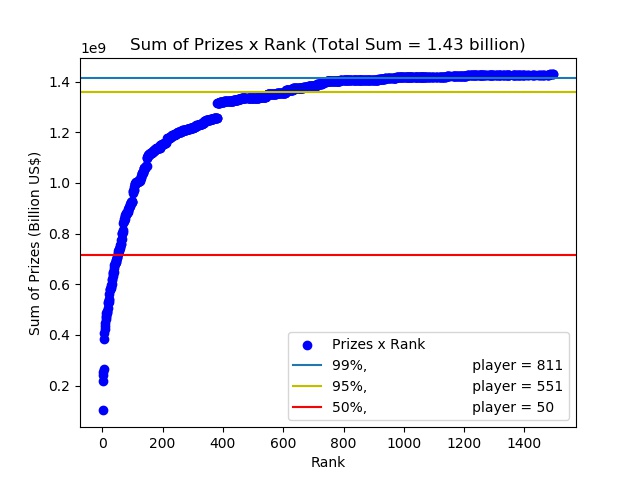
The total sum is about US$1.43 billion — damn, tennis is big — and we have 50% of that shared by only 50 players. In the ATP website, only about 2,000 players appear, but, in reality, around the world, there are more than 10,000 male professional players, giving us a 0.5% of the players controlling more than half of the prize budget, worse than society — that’s what pure competition will give you, after all, only one can be the best. Granted the curve is not as steep as expected and sponsorships are in general more valuable than prize money, the problem is not way too big, but when a low-ranked professional complains to you about his life, just give him a hug.

Now let’s analyze in more detail the problem of the bias in the weight and height for tennis players, i.e., a range of weight and height being dominant in tournaments.

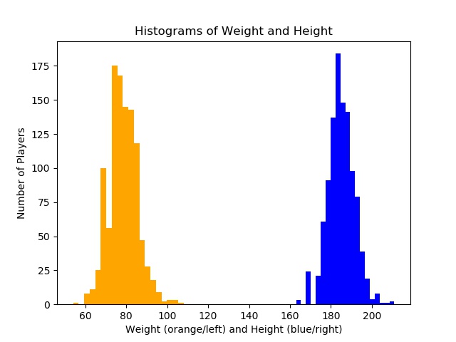
Histograms of Weight (kg) and Height (cm) for the top 1,500 players. Note that it also looks like a normal or gaussian distribution.

The histograms of weight (kg) and height (cm) make it evident that the top players are biased towards a certain weight and height: ~78 kg (172 lbs) and ~185 cm (6.06 ft ~ 6’1). To make this more clear, let’s make it two dimensional:

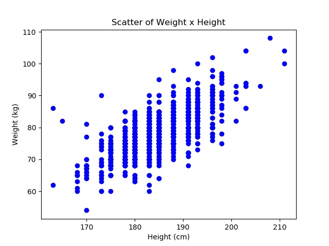
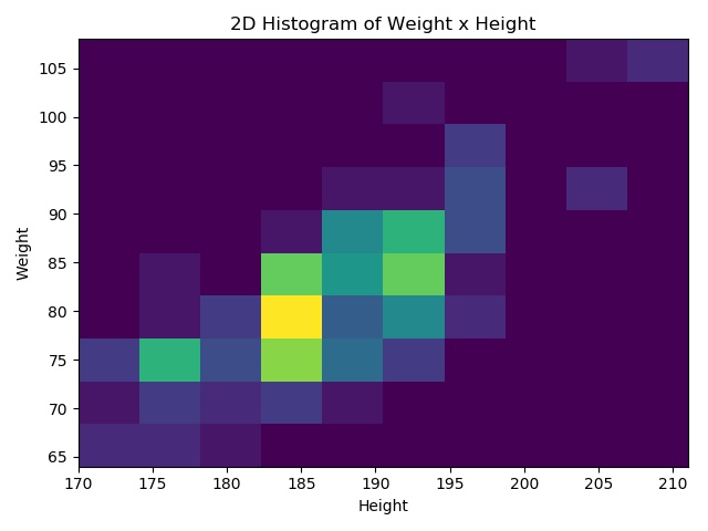
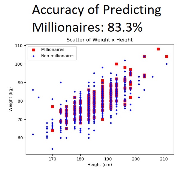
With the scatter and histogram graphs, we can see the aglomeration around the 180 cm to 195 cm and 75 kg to 90 kg. This bias gets all the more clear when you highlight the heights and weights yielding millionaires:

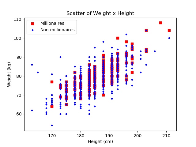
We can see that there is an internal shape to the graph, and it seems very consistent, not that many outliers. Obviously, this is not unknown to tennis players or coaches, they can usually say, by just looking at someone’s physique, if he’s going to be a successful player or not. But how good would that sort of predicament be? — i.e., what is the accuracy of that predictor?

To answer that question I wrote a script that compares four Machine Learning algorithms — Decision Trees, Support Vector Machines (SVM), K-Nearest Neighbors and Gaussian Naive Bayes; SVM and GaussianNB are almost always best in this case — to see which one gives us the best results and then averaged their performances across 500 attempts. The results are quite astonishing:

For low caps, that is, knowing if the player is going to get US$ 500,000 or more as prize money, you don’t get as good results, only 77.7% accuracy.
For medium-high caps, such as US$ 1,000,000, you start to get good predictions at 83.3% accuracy.
But the real deal starts when we put a higher cap, for example, at US$ 10,000,000: we can get up to 97% accuracy with the SVM and K-Neigh! — there isn’t that much data, so this is kind of questionable, but you get the idea.

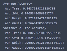
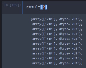
Feel free to play with the predictor and see what you could hope for if you were (or are) a tennis player. As of me, I’m glad I didn’t try tennis as a profession, because with 500 tries I still wouldn’t be a millionaire a single millionaire.

No potential for me with my 173 cm and 62 kg.

I’ll continue to post about Machine Learning and this dataset will, most likely, be used. Other even more interesting conclusions will surely come forward and I intend to put my recent Deep Learning courses to use, which will invariably yield better predictors. Also, if you spot any mistakes (I had to do so many cross-checks to get to this point…) in my code or want to suggest an improvement, feel free to message me through Facebook or initiate an issue at Github.