Telecom Nostalgia and Python Basics

Well, actually, I don’t really have much nostalgia for those days. Sorry for the clickbait title. But, in a way, the equation discussed in this post is somewhat of a good memory to me, since I find it very interesting — and its implementation turned out to teach me much more than expected, as one of the solutions involves gradient descent, the main algorithm in deep learning.

We are going to briefly discuss the Erlang Queueing functions and the B function implementation. Agner Krarup Erlang was a Danish mathematician and engineer who pioneered in the field of telecommunications. His studies innovated the field of traffic engineering and queueing theory and are still used to this day. At first applied to telephony, his queueing functions appear in many areas, most notably in calculating the size of buffers and assuring stability for networks — it can also be used for more normal queues, such as those you find in a supermarket.

The two most famous Erlang equations are probably the B and C functions:

The B function assumes a Poisson distribution for the calls and calculates the probability of blockage of a client in a system with n channels and normalized E traffic. The normalized E traffic would be:

The C function is similar, but now we calculate the probability of a delay, since the system can now have a buffer holding the delayed clients. In order to calculate the average wait time in the queue, we can use:

As an example of the impact of these functions, plugging in some values, we have that, for a system with a traffic of double its maximum capacity, i.e., E = 2, and n lines equal to 3, the average wait time is 44 units of time. If we add one more line we get an AWA of 8 units of time, a very significant cut. So, next time you go to the bank and they refuse to add another cashier out of greed, you have all the reasons to be pissed.

For the sake of brevity, in the implementation, I’ll only use the B function. It was a good exercise for learning more about Python because you can exercise the creation of classes and are almost forced to use list and dictionary comprehensions, one of the most important tools in the language. Writing code for the B function is very trivial, but the actual use of Erlang’s formulas is not so direct, our job doesn’t quite end there.

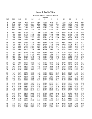
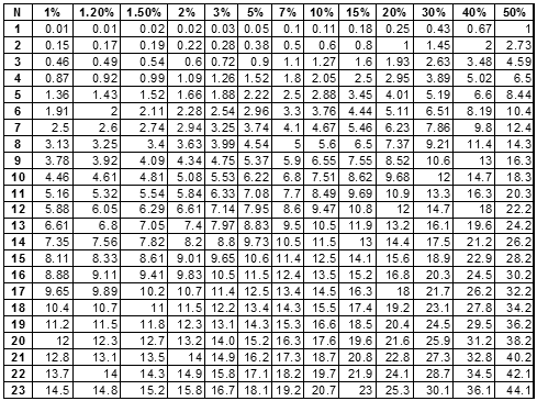
A network engineer will actually use these functions backwards, e.g., having B and E, he wants to find the number of channels n; or having B and n, he wants to find E. It turns out that isolating E or n in the formulas is not that simple analytically, therefore, we have to make use of large tables.

To find n, given B and E, is a simpler challenge since n is a discrete variable: we can just use a brute force search to solve the problem. In my code, I simply started with n=1 and iterated until I found an n which had a smaller or equal probability of blockage (the Erlang() class can assume parameters (E,1) to mimic E traffic):

        def findN_B(self, B, E):
  '''
  Finds N, given B and E,
  using the Erlang B Function
  '''
  n = 1
  while True:
    x = Erlang(E,1)
    B_found = x.B(n)
    if B_found <= B:
      return n, B_found
    else:
      n += 1
      

Looking for E, given n and B, is much more interesting — although we could have been more curious about the previous part. We have two main options to solve this problem: the first one is kind of a more intelligent brute force; and the other is gradient descent.

In the brute force solution, we would first see if the somewhat guessed solution of E yields a bigger or smaller B than the input probability. If it is bigger, we go back an arbitrary step which is equal to E minus our previous guess for E divided by 2; if it is smaller, we go forward in an analogous way. When we divide the step by 2, we are making sure the algorithm converges to the wanted E. In a way, this could be called a proto-version of Newton’s Method, and, surprisingly, this kind of dumber version of more sophisticated algorithms has been doing very well in recent years, due to their computational simplicity. For example, Monte Carlo search would be a variation of the described solution – where we randomize a value between E and our previous guess of E – and it can often find solutions to very complicated functions faster than Newton’s Method. The code for the half-stepping approach would be something like:

        def findE_B(self, n, B):
  '''
  Finds E, given n and B,
  using the Erlang B function
  '''
  E0 = 1
  eps = 0.001
  E1 = 0
  while True:
    x = Erlang(E0,1)
    B_found = x.B(n)
    if B_found - B >= eps:
      E2 = E0
      break
    else:
      E0 += 1
  while True:
    x = Erlang(E2,1)
    B_found = x.B(n)
    step = abs(E2 - E1)
    if B_found - B >= eps:
      inter = E2
      E2 -= step/2
      E1 = inter
    elif B_found - B <= -eps:
      inter = E2
      E2 += step/2
      E1 = inter
    else:
      return E2
      

The gradient descent solution is much more elegant. The spirit of it is to first declare a cost function which we would like to minimize and then make our way towards the local and global minimum of that function. Since its definition uses a convex function, a parabola embedding, we can take its derivative and apply it to our original value and be sure we are converging to the minimal cost, i.e., the E we want. The formulation is something like this:

In code, it will also look more elegant:

        def findE_B_grad(self, n, B):
  '''
  Finds E, given n and B,
  using the Erlang B function
  '''
  alpha = 0.5
  eps = 0.001
  E = 1
  while True:
    x = Erlang(E,1)
    B_found = x.B(n)
    error = abs(B_found - B)
    #Is B_found within the given error?
    if error <= eps:
      return E
    #Calculating the Derivative
    top = E**(n-1)/(np.prod(range(1,n)))
    x = [E**(i-1) for i in range(1,n+1)]
    y = [np.prod(range(1,j+1)) for j in range (1,n+1)]
    bottom = np.sum(np.divide(x,y))
    der = (B_found - B) * (top/bottom)
    
    #Gradient Descent
    E -= alpha*der
      

Unfortunately, being elegant doesn’t guarantee a solution to be the best one. This time gradient descent loses to the dumber brute search. For example, when n = 7 and B = 5%, we will have that half-stepping gets E in 1ms, while gradient descent takes 2.3s: a factor of 2300! Very disappointing! And we also have to deal with convergence/divergence problems related to the learning rate when using the gradient descent. Well, you’ve gotta test it all, before implementing one…

If you want to get all of the coding I’ve done for computing the Erlang functions — I have also included an Erlang Table Generator in the source code —, you can just visit my Github Repo, which also happens to have other algorithms I’ll be discussing in other posts. And if you want to get more info on Erlang functions, I suggest you visit this page, which has a more in-depth explanation of it, along with more related parameters.